Abstract
If Prompt Engineering designs a single model call, and Loop Engineering designs how an autonomous unit repeatedly executes, verifies and corrects its work, then Graph Engineering designs how multiple heterogeneous units depend on one another, run in parallel, converge, return for rework and receive authorisation within an executable topology.
This article argues that Graph Engineering is not simply a matter of connecting multiple Loops. Each composite node must become an evidence-constrained convergence operator. An AI Judge should therefore no longer be understood as a referee scoring candidate answers. Its task should shift to entropy assessment: recording which hypotheses a judgment adds, which possibilities it eliminates, which evidence it introduces and how much critical uncertainty remains. Nor should a local Loop aim for a monotonic decline in entropy. Its proper rhythm is entropy expansion, verification and entropy reduction: independent Judges first expose counterexamples and unknowns, experiments and evidence then update beliefs, and only then may the decision space contract on justified grounds.
Automation does not imply the exclusion of humans. A human decision is a node in the Graph with explicit inputs, outputs and routing rules, while also marking an authorisation boundary that machine optimisation cannot rewrite on its own. The AI's entropy assessment is only evidence for human judgment. Humans retain the power to confirm, reject or modify the Goal and to grant fresh authorisation. This article formalises the architecture through module quotient graphs, conditional routing, dominators, strongly connected components, graph Laplacians, Shannon entropy, KL divergence, mutual information, the data processing inequality and Fano's inequality. It also proposes an executable entropy ledger and convergence protocol.
Keywords: Loop Engineering; Graph Engineering; AI Judge; information gain; module quotient graph; human in the loop; authorisation node; auditable automation
1. How This Idea Took Shape
This line of thought did not begin with an abstract multi-agent topology. It began with the Loop Engineering architecture I had proposed earlier.
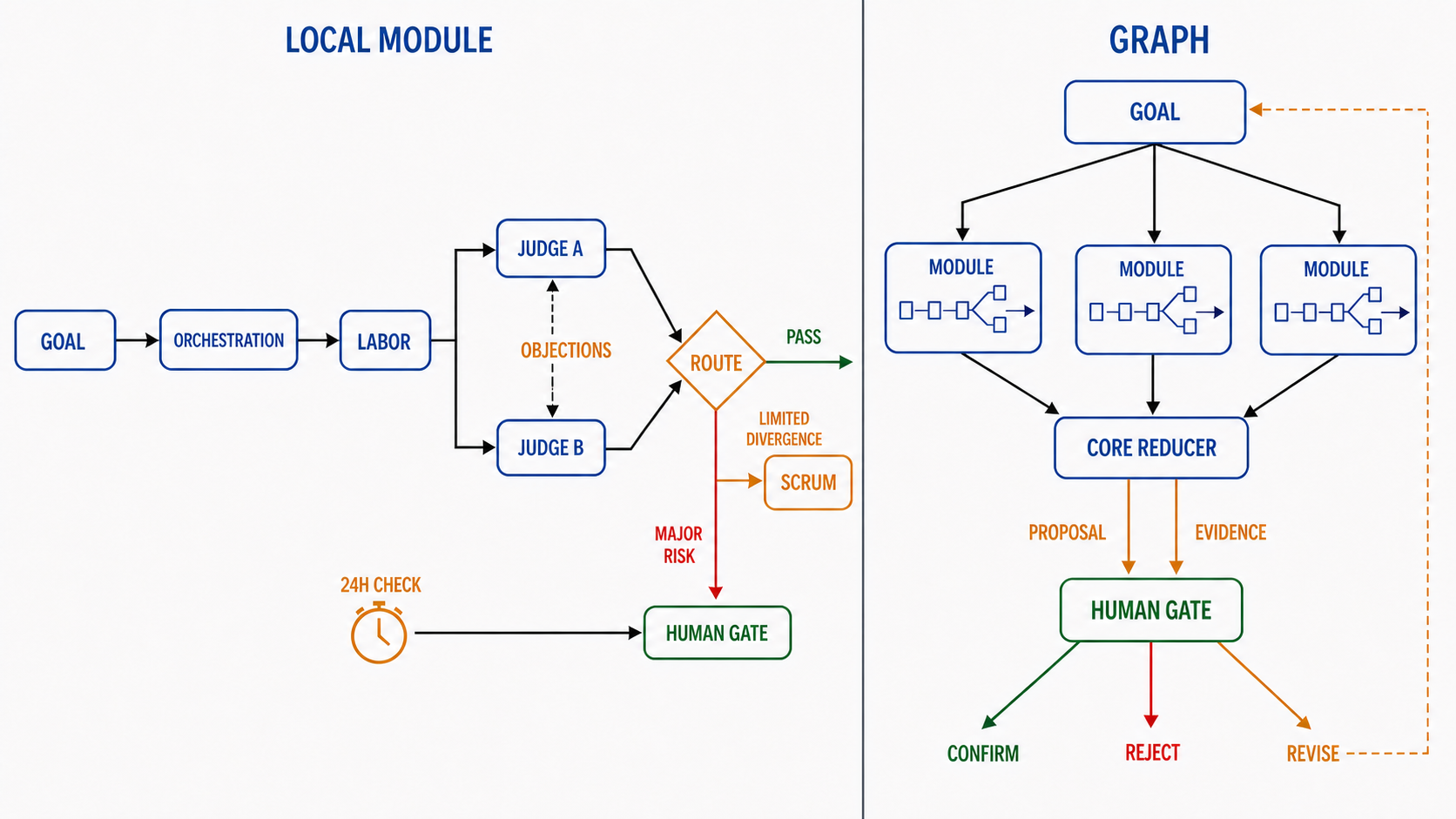
In the original structure, a human first fixes the Goal through a versioned contract. Orchestration may decompose that Goal but cannot silently rewrite it. Labor delivers artefacts that can be independently verified. Two AI Judges first assess the work separately, then exchange their strongest objections. Scrum is triggered only by disagreement, failure, risk or external change. At least once every 24 hours, the system pauses and returns to the human the authority to continue, modify, roll back or terminate the process.
The first step was to understand Graph Engineering as the layer above Loop Engineering. A Loop is no longer merely a piece of workflow code. It can become a composite node in a Graph, while many Loops are scheduled at scale through topological relationships. I then refined this view: not every node in a Graph needs to be an Agent. A node can also be a complete Loop, a deterministic function, a tool, a data source, a waiting event or a human judgment. Industry discussion since July 2026 has broadly described Graph Engineering as the explicit design of nodes, dependencies, state transitions, validation gates, recovery paths and control boundaries. It remains, however, a recent term without a single standard definition.Analytics Vidhya Both CodesDevs reflect this understanding in their definitions.
The second step was to propose a broad shape in which work converges layer by layer towards a Core Brain. The direction is sound, but it needs a boundary of authority. The Core Brain should be the final synthesiser, reducer and communicator, not a machine entity that recentralises Goal setting, execution, judgment and authorisation. It may aggregate evidence, but its topological centrality does not automatically grant it the human power to modify Goals or authorise action.
The third step produced the idea that truly changed the judgment logic. Instead of asking which opinion receives the higher score, the two AI Judges assess whether each direction can reduce uncertainty and whether their debate produces a real reduction in entropy. The Judge thereby changes from an answer scorer into a measure of convergence quality.
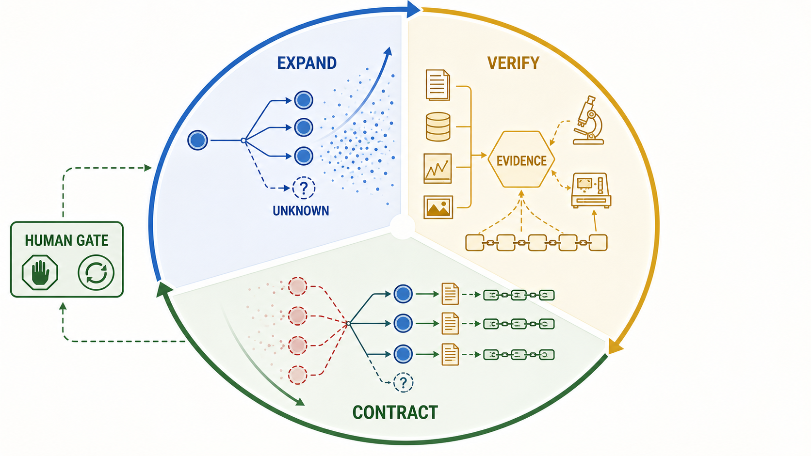
The fourth step corrected the claim that lower entropy is always better. If an adversarial Judge discovers a previously unseen risk, the system's explicit hypothesis set expands and its entropy may rise temporarily. That rise is not regression. It converts hidden ignorance into tractable uncertainty. A local Loop is therefore not a machine for monotonically reducing entropy, but a cognitive cycle that first expands entropy, then verifies, and only afterwards reduces it.
Finally, the structure gained an indispensable human node. Automation does not remove the human from the Graph. It assigns relatively simple, repetitive and verifiable work to machines, then presents the human with the evidence, residual uncertainty and risk. The human may confirm, reject or modify the machine's proposal. Humans are both inside the Graph and at the boundary of machine optimisation authority.
Together, these steps yield the central thesis of this article:
Graph Engineering is not a connection diagram of multiple Agents. It is an executable convergence system composed of local cognitive loops, evidence flows, authority flows and human authorisation nodes.
2. The Formal Object of Graph Engineering
2.1 An executable graph, not a presentation diagram
Represent an intelligent system as a directed graph with types, state and permissions:
where:
- \(V\) is the set of nodes;
- \(E\subseteq V\times V\) is the set of permitted directed transitions;
- \(\mathcal{X}\) is the global state space, including the Goal version, artefacts, evidence, risks, budget and execution history;
- \(\mathcal{T}=\{T_v\}_{v\in V}\) is the family of node state-transition operators;
- \(\Pi\) is the permission relation specifying which nodes may read, write, execute, reject or modify which states.
Nodes may be divided into:
These denote composite Loops, AI Agents, deterministic functions, tools, data nodes and human nodes. For a deterministic node, \(T_v:\mathcal{X}_{in}\to\mathcal{X}_{out}\). For a stochastic Agent, the operation may instead be written as a transition kernel:
A node is therefore not synonymous with an Agent. An Agent is one possible implementation of a node, and a complete Loop may also be encapsulated as a macroscopic node.
2.2 Edges must carry evidence and provenance
An edge should not merely say where the process goes next. It should carry a typed message:
Here, \(a\) is the artefact, \(e\) the evidence, \(p\) the provenance, \(u\) the unresolved items, \(r\) the risks, \(g\) the Goal version and \(b\) the resources consumed. Without this state, a Graph is only a flowchart, not a system that can run, recover and be audited. Recent discussions of Graph Engineering repeatedly make the same point: the difficult part is not drawing nodes and arrows, but maintaining coherent state between nodes and leaving a traceable record.Apollo Space describes this as the gap between the graph and the substrate on which it actually runs.
3. Why a Loop Can Be Treated as a Composite Node in Graph Theory
3.1 The original local topology is not a five-node circle
The original article defines a four-layer spine:
Here, \(G^{(v)}\) is the human-defined Goal version, \(O\) is Orchestration, \(L\) is Labor, \(J\) is the Dual AI Judge subgraph and \(D\) is the conditional routing node.
The Dual AI Judge is not a sequential chain \(J_A\to J_B\). When a review event is unfolded over time, the more accurate topology is:
\(J_A^{(0)}\) and \(J_B^{(0)}\) first assess the work independently. \(C_{objection}\) exchanges only their strongest objections. The two Judges may then revise their positions to \(J_A^{(1)},J_B^{(1)}\). Routing node \(D\) branches on the result:
Scrum is a conditionally triggered control point, not a stage that runs continuously during every execution. The maximum 24-hour checkpoint may also bypass Scrum and trigger the Human Gate directly. Drawing Orchestration, Labor, Judge A, Judge B and Scrum as a fixed circle therefore creates three errors at once: it turns the two Judges into a sequential dependency, makes Scrum a permanent stage and replaces conditional routing with an unconditional loop.
If Scrum decides on rework or replanning, the clearer runtime representation is to create the next versioned instance:
The unfolded graph of an individual review event can then remain a DAG, while the causal relation between versions is not obscured by an unversioned back edge.
3.2 Composite nodes depend on module partitioning, not SCC identity
Let the nodes of a local workflow be divided into disjoint modules:
Define the module quotient graph as \(Q=G/\mathcal{M}\). If there exist \(u\in M_i,v\in M_j\) such that \((u,v)\in E\), add \(M_i\to M_j\) to \(Q\). A complete Loop can become a composite node in a Graph because it has stable input, output, state and permission interfaces, not because its internal nodes must be strongly connected.
Strongly connected components remain useful, but only as a specialised tool for explicit cycles. If a workflow template retains unversioned retry edges, its SCCs can be calculated. Tarjan gave a linear-time \(O(|V|+|E|)\) algorithm in 1972.Original SIAM paper Contracting the SCCs always produces a condensation graph that is a DAG. If the condensation graph still contained a cycle, the components on that cycle would belong to one larger SCC, contradicting maximality.
A macroscopic Graph can therefore acquire a layered structure through two different routes:
- For a versioned conditional process like the one in the original article, construct the dependency DAG directly from module interfaces;
- For a workflow template with genuine explicit back edges, first condense its SCCs and then operate on the DAG between components.
The Core Brain may be represented as a convergence node \(c\) in the macroscopic DAG, but it is only a reducer:
Its outputs are proposals and evidence structures, not irrevocable authorisations.
3.3 How human nodes become verifiable authorisation gates
Let the task entry point be \(s\), a high-risk execution node be \(a\), and the set of human nodes be \(V_H\). Requiring every path from \(s\) to \(a\) to pass through some human node gives:
More strongly, if there exists \(h\in V_H\) through which every path \(s\leadsto a\) passes, then \(h\) dominates \(a\). Dominance is a standard concept in control-flow graphs, and the Lengauer-Tarjan algorithm can compute a dominator tree efficiently.Original ACM paper
The requirement that major actions pass through a human is no longer merely a line in a prompt. It becomes a topological property that can be checked statically and verified at runtime. A human node has at least three possible outputs:
confirm: authorise the downstream path under the current Goal version;reject: terminate, roll back or require rework;revise: create a new Goal version \(G^{(k+1)}\), invalidating or requiring revalidation of affected downstream conclusions.
Humans therefore have two identities. In the execution topology, a human is a node in the Graph. In the normative structure, the human is also a permission boundary that machine optimisation cannot remove on its own.
4. From Scoring to Entropy Assessment
4.1 The problem with scoring is not only subjectivity, but the wrong object of measurement
A conventional Judge often outputs:
A conclusion is then formed by averaging, weighting or majority vote. Such mechanisms compare opinions, but they do not directly represent which evidence the system has gained, which hypotheses it has eliminated or which risks it has missed.
Entropy assessment changes the object being measured. Let \(\Theta=\{\theta_1,\ldots,\theta_M\}\) be the candidate hypothesis set for the true state of the task, \(E_t\) the evidence available at time \(t\), and \(G\) the current human-authorised Goal. The belief state is:
Its Shannon entropy is:
Shannon established this information measure in 1948. Shannon entropy describes uncertainty within a given probabilistic model, but it does not directly describe semantic truth, ethical value or authorisation to act.Shannon's original paper
When a Judge or experiment produces new evidence \(Y=y\), the system performs a Bayesian update:
The information gained from one observation can be written as the KL divergence of the posterior from the prior:
Taking the expectation over possible observations gives:
This is the rigorous meaning of asking whether a line of inquiry is worth pursuing. The question is not how plausible it sounds, but how much uncertainty a verification action in that direction is expected to remove. In 1956, Lindley had already connected the information supplied by an experiment to Bayesian decision-making.Index of Lindley's original paper
4.2 Exploratory actions and final actions must be separated
For a candidate verification action \(a\), its expected information gain is:
The next verification may be selected subject to safety and budget constraints:
The final action, however, cannot be chosen by maximising information gain alone. An entirely predictable action that is certain to cause harm may also have low entropy. Final execution should therefore use utility and risk constraints:
subject to:
and, where required, explicit authorisation from some \(h\in V_H\). In other words:EIG chooses how to learn more next. The human Goal, utility and risk determine whether the system may act once it knows more.
5. Why a Sound Loop Must Pass Through Entropy Expansion, Verification and Entropy Reduction
5.1 The unknown bucket in an open world
The hypothesis set of a real task is rarely closed. Introduce an unknown state \(\bot\):
When Judge B discovers a new risk \(\theta_{m+1}\), it is making part of the probability mass in \(\bot\) explicit:
The explicit entropy may rise as a result, but the system now represents the structure of its ignorance more honestly. If this step is penalised, a Judge will be encouraged not to report new risks, producing a false appearance of low entropy.
The following illustrative example uses numbers only to explain the mechanism:
| Stage | Hypothesis distribution | Entropy (bits) | Meaning |
|---|---|---|---|
| Initial | \((0.55,0.20,0.10,0.15_{\bot})\) | 1.6815 | Three known explanations, with probability mass still assigned to the unknown |
| After Judge A | \((0.75,0.12,0.05,0.08_{\bot})\) | 1.1860 | Existing evidence supports the leading hypothesis |
| After Judge B expands entropy | \((0.60,0.10,0.04,0.08_{new},0.18_{\bot})\) | 1.6969 | A new failure mode is discovered, correcting the earlier overconfidence |
| After a targeted test | \((0.94,0.03,0.01,0.015,0.005_{\bot})\) | 0.4312 | Evidence largely rules out the new risk |
If the system rewards only entropy reduction, Judge B's contribution receives a negative value. If it records the complete cycle, it sees that Judge B prevented premature convergence.
5.2 A three-stage protocol
A local Loop should therefore distinguish three stages explicitly:
- Entropy expansion: the two Judges independently submit hypotheses, counterexamples, failure modes and unknowns, then freeze their respective records to avoid anchoring each other.
- Verification: only the strongest counterevidence and requests for evidence are exchanged. Labor, tools or external data sources perform reproducible checks.
- Entropy reduction: beliefs are updated from the evidence, unresolved objections are retained, and the system decides whether to pass, rework or escalate.
Research on multiple Judges suggests that panels of heterogeneous models can reduce within-family bias on some tasks, but this does not mean that multiple Agents are naturally more accurate.The PoLL study reported benefits from heterogeneous evaluation, while a systematic 2025 study found that multi-agent debate may substantially amplify position, verbosity, chain-of-thought and conformity biases after the first round.ACL Anthology This provides empirical support for the rule: freeze independent judgments first, then exchange counterevidence; revise in response to evidence, not in response to another model's confidence.
6. Distinguishing Real and False Entropy Reduction Mathematically
6.1 Information from two Judges cannot simply be added
Let the two Judges output \(Y_A,Y_B\). Their joint information gain follows the chain rule:
The second term is the information Judge B still adds after Judge A's output is known, not \(I(\Theta;Y_B\mid E,G)\). Therefore:
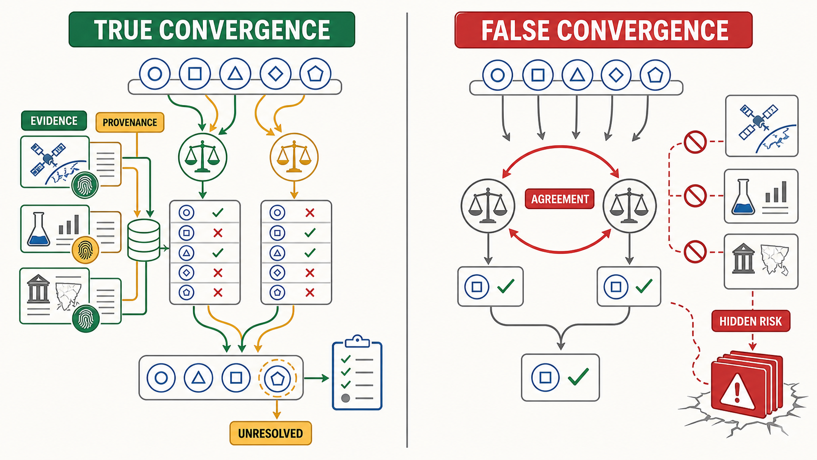
does not hold in general. If both Judges use the same model family, context and retrieval sources, their errors are highly correlated. Adding their independent scores double-counts the same evidence. An entropy-assessment system must preserve provenance and calculate conditional marginal information instead of mistaking two voices for two independent pieces of evidence.
6.2 A summary can only preserve or lose information
Let \(Y\) be the complete lower-layer evidence and \(Z=f(Y)\) the summary received by the Core Brain. If they form a Markov chain:
then the data processing inequality gives:
The Core Brain cannot create new information about the true state merely by compressing lower-layer reports. At best it preserves that information, and it will usually lose some. MIT's information-theory course materials list the data processing theorem and Fano's inequality among the foundational results.MIT OpenCourseWare
This yields a direct engineering conclusion: an upper layer cannot receive only a single word such as PASS or a numerical score. Its summary must carry references to the original evidence, objections and eliminated hypotheses. Otherwise, cross-layer aggregation will systematically discard information.
6.3 Why low residual entropy still does not imply correctness
For \(M\) candidate hypotheses and any estimator \(\hat\Theta(Z)\), let the probability of error be \(P_e\). Fano's inequality gives:
where \(h_b\) is the binary entropy function. The inequality shows that classification error cannot generally be low when conditional entropy is high. Its converse, however, must not be misused. Low entropy does not automatically guarantee correctness, especially when:
- the truth lies outside the hypothesis space;
- the probabilities are uncalibrated confidence claims reported by a language model;
- the evidence is wrong or contaminated;
- multiple Judges share the same bias;
- the system lowers entropy by deleting objections rather than resolving them.
Entropy is therefore a measure of epistemic uncertainty, not a correctness score and certainly not a substitute for value or authorisation.
7. Put Humans in the Graph, Not in Exception Handling
7.1 The goal of automation is not to maximise the share of machine nodes
If automation means avoiding human involvement wherever possible, human intervention is treated as failure, delay or cost. In a human-governed Graph Engineering system, the proper objective should instead be:
subject to:
AI is suited to repetitive execution, search, organisation, preliminary verification and evidence compression. Human nodes handle value conflicts, Goal modification, irreversible actions, major tail risks and information outside the model. Human intervention is not the opposite of automation. It is part of automation's permission structure.
7.2 Humans impose an external constraint on entropy assessment
The AI should present the human not with a single recommendation, but with a decision certificate:
It contains the current Goal version, candidate hypotheses, probabilities or structured support, evidence, information gain, unresolved items, risks, rollback conditions and provenance.
The human may judge from \(\mathcal{C}\), but may also introduce a new variable \(Z_H\) absent from the machine's model, thereby changing the hypothesis space or utility function:
This step cannot be interpreted as adding a human-weighted entropy score to the AI's calculation. The human holds meta-authority to change the problem definition and the authorisation boundary, not merely one ordinary vote on an evaluation panel.
8. An Executable Dual-Judge Entropy-Ledger Protocol
At round \(k\), each local Loop maintains the state:
where \(U_k\) is the set of unresolved propositions, \(R_k\) the set of risks, \(B_k\) the remaining budget and \(P_k\) the evidence-provenance graph.
Rather than returning a single overall score, each Judge outputs:
EntropyLedger {
  goal_version
  prior_hypotheses
  newly_exposed_hypotheses
  evidence_added
  hypotheses_eliminated_with_evidence
  surviving_hypotheses
  unresolved_contradictions
  critical_tail_risks
  provenance
  requested_tests
  proposed_action
  rollback_conditions
}
The protocol is as follows:
- Judge A and Judge B submit and freeze their ledgers independently, without seeing the other's conclusion;
- merge new hypotheses, but do not merge duplicate evidence;
- calculate the conditional marginal information gain of each piece of evidence;
- the two Judges exchange only their strongest counterevidence and the tests they require;
- Labor or external tools execute those tests;
- update \(p_k\) using a joint likelihood, not a false assumption of conditional independence;
- produce the new residual uncertainty, risks and objections;
- submit to the upper layer if the pass conditions are met, otherwise rework or enter a human node.
A more robust pass condition is a conjunction of constraints, not a single threshold:
Here, \(D_G\) measures how far machine execution has drifted from the human-authorised Goal. No major risk should be averaged away because other dimensions perform well.
For open-ended tasks without reliable probabilities, an operational convergence vector may be used:
Use a Pareto order rather than forcing the vector into a single score. Structural progress occurs only if \(\mathbf{q}'\) is no worse than \(\mathbf{q}\) on every critical dimension and strictly better on at least one.
9. How Local Convergence Becomes Global Convergence
9.1 Local information gains cannot simply be summed
Suppose a macroscopic Graph contains \(m\) Loops producing evidence \(Y_1,…,Y_m\). The global information is:
This is a sum of conditional gains, not a simple sum of each node's independent information gain. The expression yields three engineering requirements:
- The Graph must record dependencies between evidence to prevent double-counting;
- node order affects the interpretation of marginal contribution but does not change the joint mutual information;
- the Core Brain must see provenance and correlation, not merely local scores.
9.2 A cycle-level potential function
Define a global potential function at the end of each complete Loop cycle:
The entropy-expansion phase may temporarily raise \(\Psi\), so comparisons are made only at complete cycle boundaries. If every cycle that has not stopped satisfies:
then after at most
effective contraction cycles, the system must either reach its target threshold or trigger a budget stop or human escalation. This gives a finite-step guarantee against endless discussion.
The proposition guarantees only termination under the specified potential function. It does not prove that the conclusion must be correct. Correctness still depends on the hypothesis space, evidence quality, model calibration and the human Goal. This is the boundary of what graph theory and information theory can provide: they can establish topological and update properties, but they cannot decide what the system ought to pursue.
9.3 Insights and limits of consensus dynamics
In a linear multi-agent consensus model, node states \(x\in\mathbb{R}^n\) may be updated through the graph Laplacian \(L\):
For a connected undirected graph, the second-smallest eigenvalue of \(L\) satisfies \(\lambda_2(L)>0\), and the system can converge asymptotically to the consensus space. \(\lambda_2\) is also related to the convergence rate. The survey by Olfati-Saber, Fax and Murray gives a systematic account of graph structure, Laplacian spectra and multi-agent consensus.Original technical report
Agreement of opinion means only that \(x_i-x_j\to0\), not that \(x_i\to\theta^*\). If every node shares the same error, a system can converge rapidly on a false consensus. In an AI Judge system, consensus in the Laplacian sense is therefore only a coordination property. Convergence towards truth still requires anchors in external evidence and human constraints.
10. What the Core Brain Should Be
The most dangerous definition of a Core Brain is a super-Agent that ultimately possesses all information and authority. Such a design recombines the four powers that Loop Engineering deliberately separated: Goal setting, task execution, result judgment and authorisation to continue.
A more appropriate Core Brain is a constrained reduction core:
It should satisfy the following requirements:
- it cannot silently rewrite the Goal version;
- it cannot delete provenance or objections;
- it cannot count correlated evidence more than once;
- it cannot conceal major tail risks within an overall average;
- it cannot bypass a human node that dominates a high-risk path;
- it can generate proposals only, while final authorisation follows the permission graph.
Convergence towards the Core Brain remains possible under this definition, but what converges is information and proposed action, not human sovereignty.
11. Falsifiability Boundaries and Engineering Risks
This model still has several limits that must be acknowledged directly.
First, entropy must be defined over explicit random variables and a hypothesis space. Without \(\Theta\) and a probabilistic model, an entropy value is only a metaphor. Open-ended tasks may use a structured uncertainty vector, but should not present it as Shannon entropy.
Second, a model's self-reported confidence is not a calibrated probability. Calibration requires historical data, external tests, repeated sampling or an explicit likelihood model. Otherwise, KL divergence merely calculates an unreliable distribution with precision.
Third, heterogeneity among Judges must be genuine. Different role prompts may still produce highly correlated errors if the Judges share the same model, training corpus and retrieval sources.
Fourth, entropy reduction is vulnerable to Goodhart's law. Once entropy reduction becomes a reward, a system may optimise the metric by deleting difficult hypotheses, suppressing objections or becoming overconfident. Hypothesis coverage, evidence provenance and unknown probability mass must therefore be audited alongside it.
Fifth, human judgment is also fallible. Treating humans as authorisation nodes does not assume that humans are omniscient. It recognises that responsibility for values, Goal modification and irreversible action cannot be hidden inside a machine score. Systems with multiple human nodes also need explicit permission graphs, conflict resolution and accountability instead of falling back once again on a simple majority vote.
Conclusion: Graph Engineering as Distributed Cognitive Governance
The real change from Loops to Graphs is not an increase in the number of Agents. It is the entry of local autonomous units into an integrated structure with dependencies, evidence, permissions and recovery paths.
The real change from scoring to entropy assessment is likewise not the replacement of a hundred-point scale with a more sophisticated number. It changes what a Judge measures. The question is no longer whose opinion looks most like a winner, but what the system has learned from the judgment, what it has ruled out and which unknowns it has honestly exposed.
Writing humans into the Graph means that automation finally ceases to define its purpose as excluding people. Machines perform repeatable cognitive labour. Entropy assessment makes uncertainty visible. The Core Brain integrates evidence and forms proposals. Human nodes retain the authority to confirm, reject, modify and reauthorise.
The architecture can therefore be compressed into three layers:
Graph Engineering is no longer merely a technique for orchestrating workflows. It becomes a form of distributed cognitive governance, managing not only how machines work, but also how a system acknowledges the unknown, forms judgments and determines who has the authority to turn judgment into action.
References
- Claude E. Shannon, A Mathematical Theory of Communication, 1948.
- D. V. Lindley, On a Measure of the Information Provided by an Experiment, 1956.
- Robert Tarjan, Depth-First Search and Linear Graph Algorithms, SIAM Journal on Computing, 1972.
- Thomas Lengauer and Robert E. Tarjan, A Fast Algorithm for Finding Dominators in a Flowgraph, ACM TOPLAS, 1979.
- Reza Olfati-Saber, J. Alex Fax, Richard M. Murray, Consensus and Cooperation in Networked Multi-Agent Systems, Proceedings of the IEEE, 2007.
- Pat Verga et al., Replacing Judges with Juries: Evaluating LLM Generations with a Panel of Diverse Models, 2024.
- Chiyu Ma et al., Judging with Many Minds: Do More Perspectives Mean Less Prejudice?, Findings of EMNLP, 2025.
- MIT OpenCourseWare, Information Theory: Data Processing Theorem and Fano’s Inequality.
- Fathin Dosunmu, Graph Engineering for AI Agents: What It Is and When to Use It, 2026.
- Harsh Mishra, Graph Engineering for AI Agents: Beyond the Single-Agent Loop, 2026.
Note on the origin of the ideas
The original Loop Engineering architecture, in which humans set a versioned Goal, Orchestration decomposes it, Labor executes it, two AI Judges review independently before examining each other's objections, Scrum is invoked as needed, and humans reauthorise the work at least once every 24 hours, was proposed by Suxi’s World in an earlier article.
In developing this article, Suxi further articulated three central ideas: Graph Engineering can aggregate complete Loops layer by layer as composite nodes; Judges should move from scoring opinions to assessing uncertainty; and human decision-making is not an exception to automation but an indispensable authorisation node in the Graph. Suxi then corrected the mistaken diagram of a local Loop as a five-node circle, reaffirming its actual structure as a linear spine, two Judges that begin independently and couple only later, conditionally triggered Scrum and human escalation. The module quotient graph, conditional routing, dominance relation, information gain, distinction between real and false entropy reduction, and potential function are mathematical formalisations developed around these ideas.